深度学习卷积神经网络(斯坦福2016 CS231n)笔记

CS231n Lecture 3 第三个视频笔记

SVM && Softmax && Learning Rates && Gradient Check && Mini-batch Gradient Descent

SVM loss function

def L_i_vector(x,y,W):
	scores = W.dot(x)
	margins = np.maximum(0,scores - scores[y]+1)
	margins[y] = 0   #只是为了不等于1
	loss_i = np.sum(margins)
	return loss_i

Regularization motivation

Take all X into account

lambda.dot(R(W))

R(w)可能情况

L2 regularization: R(W) = square(W)

L1 regularization: R(W) = abs(W) — feature selection

Elastic net(L1+L2):R(W) = \beta.dot(W.dot(W)) + abs(W)

Max norm regularization

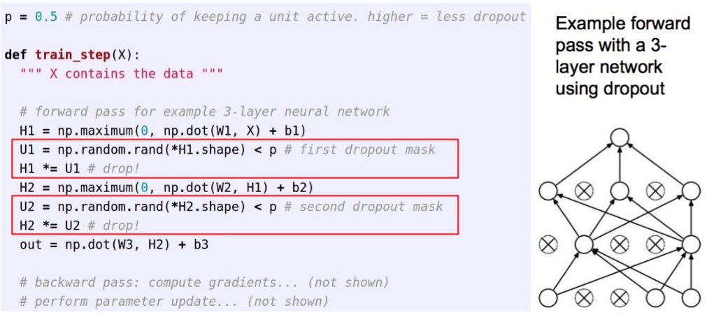
Dropout

Softmax Classifier(Multinomial Logistic Regression)

scores = unnormalized log probabilities of the classes.

$P(Y=k \| X=xi) = \frac{e^{S_k}}{\sum_j e^{S_j})} ;S = f(x_i;W,b)) = W x_i + b$

maximize the log likelihood or minimize the negative log likelihood

Loss: Li = -log(P(Y=yi|X=xi))

Softmax vs. SVM

if changing its score slightly,SVM doesn’t care.Softmax will change a lot.

$L = \frac{1}{N} \sum_i \sum_{j \neq y_i} \max(0,f_j - f_{y_i} + 1) + \lambda \sum_k \sum_l W_{k,l}^2$ $L = \underbrace { \frac{1}{N} \sum_i \sum_{j \neq y_i} \max(0,f_j - f_{y_i} + 1)}_{\text{data loss}} + \lambda \underbrace{\sum_k \sum_l W_{k,l}^2}_{\text{regularization loss}}$

CS231n Lecture 4 第四个视频 BP & NN

Chain rule

calc $ f(x,y,z) = (x+y)z $ to understand activations of backprop.

Another large example:

$f(w,x) = \frac{1}{1+e^{-(w_0 x_0 + w_1 x_1 + w_2)}}$

Jacobian Matrix Diagonal Sparsity

NN

超厉害的11行代码实现两层神经网络 Basic Python Network

X = np.array([ [0,0,1],[0,1,1],[1,0,1],[1,1,1] ])
y = np.array([[0,1,1,0]]).T
syn0 = 2*np.random.random((3,4)) - 1	#Weight  Synapse 突触
syn1 = 2*np.random.random((4,1)) - 1
for j in xrange(60000):
    l1 = 1/(1+np.exp(-(np.dot(X,syn0))))
    l2 = 1/(1+np.exp(-(np.dot(l1,syn1))))
    l2_delta = (y - l2)*(l2*(1-l2))
    l1_delta = l2_delta.dot(syn1.T) * (l1 * (1-l1))
    syn1 += l1.T.dot(l2_delta)
    syn0 += X.T.dot(l1_delta)

Cell body : sum && bias

Activation funtion

sigmoid

tanh(x):$ tanh(x) $

ReLU:$max(0,x)$ make your classifier more faster, use as default

Leaky ReLU: $max(0.1 x,x) $

Maxout: $ max(w_1^T x +b_1,w_2^T x +b_2) $

ELU:$ f(x) = \left{\begin{array}{c} x
\alpha (e^x-1) \end{array} \right. $

NN

数layers时，input layer不算

非常有意思的演示，将空间的转变演示出来了

More always better~but you need avoid overfiting

不同的layer不同的function，一般没人这么做

Lecture 5 NN part2

ConvNets 并不一定需要大量数据—— finetuning

Don’t be overly ambitious.

Train NN

Loop:

Sample a batch of data
Forward prop it through the graph, get loss
Backprop to calculate the gradients
Update the parameters using the gradient

Training Neural Networks

One time setup

activation functions, preprocessing, weight initialization, regularization, gradient checking

Training dynamics

babysitting the learning process, parameter updates, hyperparameter optimization

Evaluation

model ensembles

Activation functions

Sigmoid funcition

[0,1]

Problem: downside 1. Saturated neurons “kill” the gradients

x 在 -10 ,10之外的时候，好多节点就无法传递BP的gradients了

Sigmoid outputs are not zero-centered

$ W_i $ Always all positive or all negative

none-zero-centered function converge slower

exp() is a bit compute expensive

Tanh(x)

[-1,1] zero-centered

Problem: 1. also Saturated

ReLu

$f(x) = max(0,x)$

2012年的时候才解释==

Don’t saturate (in +region)
Very computationally efficient
Converges much faster than sigmoid/tanh

Problems: 1. not zero-centered output 2. An annoyance: When x<=0 , gradient is killed.问题是，初始化的时候初始化的不好，最后就会有几个Neuron从来没有Updated过。最后就是相当于Dead Neuron，数据从来没经历过这些节点。（常见解决方法（可能不管用）：初始化的时候with slightly positive bias eg:0.01）

Leaky ReLU

为了解决ReLU里面的dead Neuron的问题

$f(x) = max(0.01 x,x)$ $f(x) = max(\alpha x,x)$

Will not ‘die’

ELU exponential linear units

$f(x) = \begin{cases} x, & \text{if $x > 0$} \\ \alpha (e^x-1), & \text{if $x \leq 0$} \\ \end{cases}$

2015年10月份的。。。。。[Clevert et al., 2015] 2页paper来证明。。

Maxout

$max(w_1^T x +b_1,w_2^T x +b_2)$

[Goodfellow et al., 2013]

Does not have the basic form of dot product -> nonlinearity
Generalizes ReLU and Leaky ReLU
Linear Regime! Does not saturate! Does not die!

Problem: doubles the number of parameters/neuron :(

Important!!!

Use ReLU. Be careful with your learning rates
Try out Leaky ReLU / Maxout / ELU
Try out tanh but don’t expect much
Don’t use sigmoid

Data Preprocessing

常用的就是Zero-center，一般不用normalize 或者 PCA或者whitening

Not common to normalize variance, to do PCA or whitening

In practice for Images: center only

Subtract the mean image (e.g. AlexNet)
Subtract per-channel mean (e.g. VGGNet)

Weight Initialization

Tiny number的话，最后W会很小

如果超级混乱的init，disaster

（linear activations）合理的Init

“Xavier initialization” [Glorot et al., 2010]

W = np.random.randn(fan_in,fan_out) / np.sqrt(fan_in)
# but when using the ReLU nonlinearity it breaks.

Layer std decrease

对于 ReLU

[He et al., 2015] note additional /2

W = np.random.randn(fan_in,fan_out) / np.sqrt(fan_in / 2)

论文

Understanding the difficulty of training deep feedforward neural networks by Glorot and Bengio, 2010

Exact solutions to the nonlinear dynamics of learning in deep linear neural networks by Saxe et al, 2013

Random walk initialization for training very deep feedforward networks by Sussillo and Abbott, 2014

Delving deep into rectifiers: Surpassing human-level performance on ImageNet classification by He et al., 2015

Data-dependent Initializations of Convolutional Neural Networks by Krähenbühl et al., 2015

All you need is a good init, Mishkin and Matas, 2015

Batch Normalization

[Ioffe and Szegedy, 2015]

“you want unit gaussian activations? just make them so.”

Usually inserted after Fully Connected(FC) / (or Convolutional, as we’ll see soon) layers, and before nonlinearity.

Improves gradient flow through the network
Allows higher learning rates
Reduces the strong dependence on initialization
Acts as a form of regularization in a funny way, and slightly reduces the need for dropout, maybe

可能有30%的速度衰减

什么时候用BN？

Babysitting the Learning Process

Preprocess the data
Choose the architecture

Make sure that you can overfit very small portion of the training data

Learning rate = 1e-6,直接用眼看

cost: NaN almost always means high learning rate…

Hyperparameter Optimization

change range to calc learning rate

Grid Search vs random Search

Always use random search

Loss function

http://lossfunctions.tumblr.com/

big gap = overfitting => increase regularization strength?

no gap => increase model capacity?

Track the ratio of weight updates / weight magnitudes:

ratio between the values and updates: ~ 0.0002 / 0.02 = 0.01 (about okay) want this to be somewhere around 0.001 or so

Important！！

Regularization (Dropout etc)
Evaluation (Ensembles etc)

Lecture 6 NN

full saturated or all zeros

Parameter update schemes
Learning rate schedules
Dropout
Gradient checking
Model ensembles

Parameter update

SGD is so slow

SGD is a very slow progress along flat direction, jitter along steep one

Momentum update

比SGD快

v = mu * v - learning_rate * dx
X += v

解释

Physical interpretation as ball rolling down the loss function + friction (mu coefficient).
mu = usually ~0.5, 0.9, or 0.99 (Sometimes a

优势

Allows a velocity to “build up” along shallow directions
Velocity becomes damped in steep direction due to quickly changing sign

Nesterov Momentum update (nag)

“lookahead” gradient step (bit different than original)

$v_t = u v_{t-1} - \epsilon \nabla f(\phi_{t-1}) \phi_t = \phi_{t-1} - \mu v_{t-1} + ( 1 + \mu ) v_t$

v_prev = v
v = mu * v - learning_rate * dx
X += -mu * v_prev + (1+mu)*v

** Common commercial network!!!!!!!**

AdaGrad update

cache += dx ** 2
x += - learning_rate * dx / (np.sqrt(cache)+1e-7)

Added element-wise scaling of the gradient based on the historical sum of squares in each dimension

相当于自动变化Learning Rate

现实中并不是这么好，到最后可能导致lr更大

RMSProp update

[Tieleman and Hinton, 2012]

cache += decay_rate * cache + (1 - decay_rate) * dx ** 2
x += - learning_rate * dx / (np.sqrt(cache)+1e-7)

Adam update

合并了RMSProp和Momentum

[Kingma and Ba, 2014]

m,v = #... initialize caches to zeros
for t in xrange(0,big_number):
	dx = # evalute gradient
	m = beta1*m + (1-beta1)*dx
	v = beta2*v + (1-beta2)*(dx**2)
	m /= 1 - beta1**t
	v /= 1 - beta2**t
	x += - learning_rate * m / (np.sqrt(v) + 1e-7)

用这个比较多

learning rate as a hyperparameter

Step decay
exponential decay
1/t decay

Second order optimization methods

使用了 Hessian，Invert the Hessian($O(n^3)$)

BGFS 把inverse Hessian with rank 1 优化成 $O(n^2)$
L-BGFS Does not form/store the full inverse Hessian.

L-BGFS

very heavy function. In practice,we don’t use it.

Usually works very well in full batch, deterministic mode. i.e. if you have a single, deterministic f(x) then L-BFGS will probably work very nicely
Does not transfer very well to mini-batch setting. Gives bad results. Adapting L-BFGS to large-scale, stochastic setting is an active area of research.

In practice

Adam is a good default choice in most cases
If you can afford to do full batch updates then try out L-BFGS (and don’t forget to disable all sources of noise) 一般不用

Evaluation

经验

Train multiple independent models
At test time average their results

Enjoy 2% extra performance

??????????????

can also get a small boost from averaging multiple model checkpoints of a single model.
keep track of (and use at test time) a running average parameter vector:

Regularization(Dropout)

dropout

why use dropout

Forces the network to have a redundant representation.
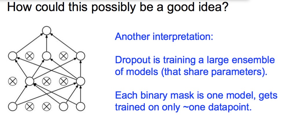
Dropout is training a large ensemble of models (that share parameters).
Each binary mask is one model, gets trained on only ~one datapoint.

In practice

drop的时候要注意

Leave all input neurons turned on (no dropout).
With p=0.5, using all inputs in the forward pass would inflate the activations by 2x from what the network was “used to” during training! => Have to compensate by scaling the activations back down by 1⁄2

???????

ConvNets Face recognize [Taigman et al. 2014]

Deep Neural Networks Rival the Representation of Primate IT Cortex for Core Visual Object Recognition [Cadieu et al., 2014]